This page was generated by nbsphinx from docs/notebooks/transform/LaPD6KTransform.ipynb.

Demo of LaPD6KTransform

%matplotlib inline

import numpy as np
import matplotlib.pyplot as plt
import sys

plt.rcParams["figure.figsize"] = [10.5, 0.56 * 10.5]

try:
    from bapsf_motion.transform import LaPD6KTransform
except ModuleNotFoundError:
    from pathlib import Path

    HERE = Path().cwd()
    BAPSF_MOTION = (HERE / ".." / ".." / ".." ).resolve()
    sys.path.append(str(BAPSF_MOTION))

    from bapsf_motion.transform import LaPD6KTransform

General input keyword arguments to use for the demo.

input_kwargs = {
    "pivot_to_center": 57.288,
    "pivot_to_drive": 134.0,
    "pivot_to_feedthru": 21.6,
    "probe_axis_offset": 20.1,
    "droop_correct": False,
}

Transform from Motion Space to Drive Space to Motion Space

Let’s show the transform can successfully convert from the motion space to the drive space, and back.

Instantiate the transform class.

tr = LaPD6KTransform(("x", "y"), **input_kwargs)
tr.config

{'type': 'lapd_6k',
 'pivot_to_drive': 134.0,
 'pivot_to_feedthru': 21.6,
 'drive_polarity': [1, -1],
 'droop_scale': 1.0,
 'six_k_arm_length': 93.345,
 'mspace_polarity': [-1, 1],
 'probe_axis_offset': 20.1,
 'pivot_to_center': 57.288,
 'droop_correct': False}

Construct a set of points in the motion space to convert.

points = np.zeros((40, 2))
points[0:10, 0] = np.linspace(-5, 5, num=10, endpoint=False)
points[0:10, 1] = 5 * np.ones(10)
points[10:20, 0] = 5 * np.ones(10)
points[10:20, 1] = np.linspace(5, -5, num=10, endpoint=False)
points[20:30, 0] = np.linspace(5, -5, num=10, endpoint=False)
points[20:30, 1] = -5 * np.ones(10)
points[30:40, 0] = -5 * np.ones(10)
points[30:40, 1] = np.linspace(-5, 5, num=10, endpoint=False)

key_points = np.array(
    [
        [-5, 5],
        [-5, -5],
        [5, -5],
        [5, 5],
        [0, 0]
    ],
)

Calculate the drive space points dpoints and return to motion space points mpoints.

dpoints = tr(points, to_coords="drive")
mpoints = tr(dpoints, to_coords="motion_space")

Plot the transform

figwidth, figheight = plt.rcParams["figure.figsize"]
figwidth = 1.4 * figwidth
figheight = figheight
fig, axs = plt.subplots(1, 3, figsize=[figwidth, figheight])

axs[0].set_title("Motion Space")
axs[1].set_title("Drive Space")
axs[2].set_title("Motion Space Return")

for ii in range(3):
    axs[ii].set_xlabel("X")
    axs[ii].set_ylabel("Y")

axs[0].fill(points[...,0], points[...,1])
axs[1].fill(dpoints[...,0], dpoints[...,1])
axs[2].fill(mpoints[...,0], mpoints[...,1])

for pt, color in zip(
    key_points.tolist(),
    ["red", "orange", "green", "purple", "black"]
):
    dpt = tr(pt, to_coords="drive")
    mpt = tr(dpt, to_coords="motion_space")
    axs[0].plot(pt[0], pt[1], 'o', color=color)
    axs[1].plot(dpt[..., 0], dpt[..., 1], 'o', color=color)
    axs[2].plot(mpt[..., 0], mpt[..., 1], 'o', color=color)

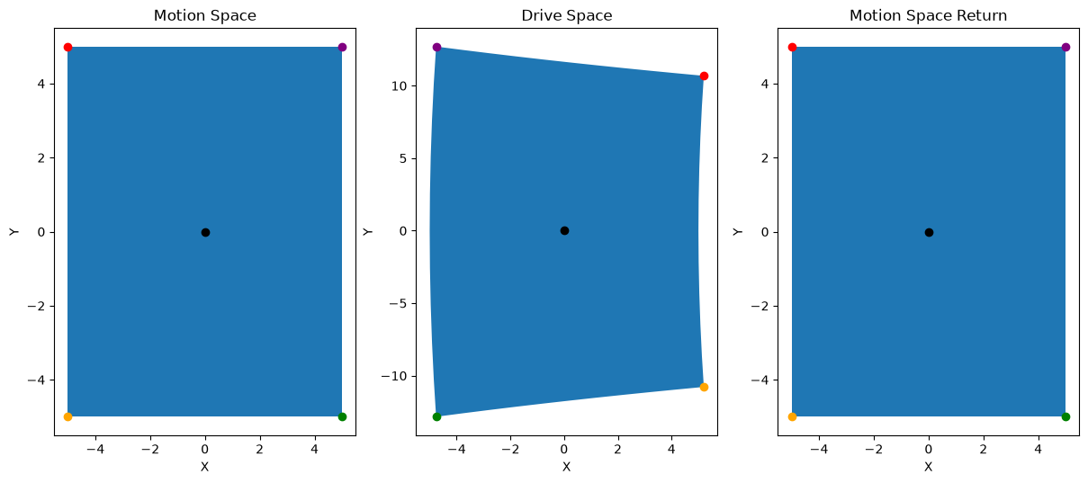
Are the returned motion space points “identical” to the starting points?

np.allclose(points, mpoints)

True

np.max(np.abs(points - mpoints))

np.float64(2.0872192862952943e-14)

Transform from Drive Sapce to Motion Space to Drive Space

Let’s show the transform can successfully convert from the drive space to the motion space, and back.

Using the same transform and initial points in the previous section, lets construct the motion space points mpoints and return to drive space points dpoints.

mpoints = tr(points, to_coords="motion_space")
dpoints = tr(mpoints, to_coords="drive")

Plot the transform.

figwidth, figheight = plt.rcParams["figure.figsize"]
figwidth = 1.4 * figwidth
figheight = figheight
fig, axs = plt.subplots(1, 3, figsize=[figwidth, figheight])

axs[0].set_title("Drive Space")
axs[1].set_title("Motion Space")
axs[2].set_title("Drive Space Return")

for ii in range(3):
    axs[ii].set_xlabel("X")
    axs[ii].set_ylabel("Y")

axs[0].fill(points[...,0], points[...,1])
axs[1].fill(mpoints[...,0], mpoints[...,1])
axs[2].fill(dpoints[...,0], dpoints[...,1])

for pt, color in zip(
    key_points.tolist(),
    ["red", "orange", "green", "purple", "black"]
):
    mpt = tr(pt, to_coords="motion_space")
    dpt = tr(mpt, to_coords="drive")
    axs[0].plot(pt[0], pt[1], 'o', color=color)
    axs[1].plot(mpt[..., 0], mpt[..., 1], 'o', color=color)
    axs[2].plot(dpt[..., 0], dpt[..., 1], 'o', color=color)

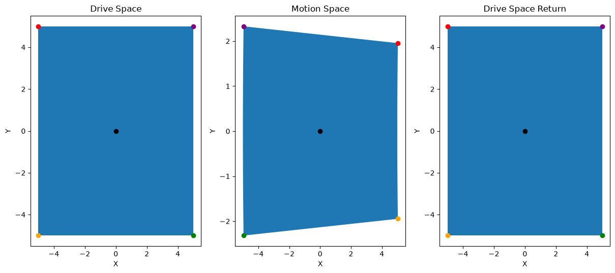
Are the returned drive space points “identical” to the starting points?

np.allclose(points, dpoints)

True

np.max(np.abs(points - dpoints))

np.float64(3.552713678800501e-14)

Transform Can Droop Correct

The transform LaPD6KTransform also incorporates droop correction via the LaPDXYDroopCorrect class.

Instantiate the transform with droop correction enabled.

tr = LaPD6KTransform(
    ("x", "y"),
    **{
        **input_kwargs,
        "droop_correct": True,
        "droop_scale": 2.0,
    },
)
tr.config

{'type': 'lapd_6k',
 'pivot_to_drive': 134.0,
 'pivot_to_feedthru': 21.6,
 'drive_polarity': [1, -1],
 'droop_scale': 2.0,
 'six_k_arm_length': 93.345,
 'mspace_polarity': [-1, 1],
 'probe_axis_offset': 20.1,
 'pivot_to_center': 57.288,
 'droop_correct': True}

Construct a set of points for the transform.

points = np.zeros((40, 2))
points[0:10, 0] = np.linspace(-5, 5, num=10, endpoint=False)
points[0:10, 1] = 5 * np.ones(10)
points[10:20, 0] = 5 * np.ones(10)
points[10:20, 1] = np.linspace(5, -5, num=10, endpoint=False)
points[20:30, 0] = np.linspace(5, -5, num=10, endpoint=False)
points[20:30, 1] = -5 * np.ones(10)
points[30:40, 0] = -5 * np.ones(10)
points[30:40, 1] = np.linspace(-5, 5, num=10, endpoint=False)

key_points = np.array(
    [
        [-5, 5],
        [-5, -5],
        [5, -5],
        [5, 5],
        [0, 0]
    ],
)

Calculate the drive space points dpoints and return to motion space pointsmpoints.

dpoints = tr(points, to_coords="drive")
mpoints = tr(dpoints, to_coords="motion_space")

Plot the transform.

figwidth, figheight = plt.rcParams["figure.figsize"]
figwidth = 1.4 * figwidth
figheight = figheight
fig, axs = plt.subplots(1, 3, figsize=[figwidth, figheight])

axs[0].set_title("Motion Space")
axs[1].set_title("Drive Space")
axs[2].set_title("Motion Space Return")

for ii in range(3):
    axs[ii].set_xlabel("X")
    axs[ii].set_ylabel("Y")

axs[0].fill(points[...,0], points[...,1])
axs[1].fill(dpoints[...,0], dpoints[...,1])
axs[2].fill(mpoints[...,0], mpoints[...,1])

for pt, color in zip(
    key_points.tolist(),
    ["red", "orange", "green", "purple", "black"]
):
    dpt = tr(pt, to_coords="drive")
    mpt = tr(dpt, to_coords="motion_space")
    axs[0].plot(pt[0], pt[1], 'o', color=color)
    axs[1].plot(dpt[..., 0], dpt[..., 1], 'o', color=color)
    axs[2].plot(mpt[..., 0], mpt[..., 1], 'o', color=color)

Are the returned motion space points “identical” to the starting points?

np.allclose(points, mpoints)

True

np.max(np.abs(points - mpoints))

np.float64(3.632436573752784e-10)

Configure for West Side Deployment

The default values for LaPD6KTransform is for an East side deployment on the LaPD. However, the transform can be configured for a West side deployment by using a negative pivot_to_center and [1, 1] for the mspace_polarity.

tr = LaPD6KTransform(
    ("x", "y"),
    **{
        **input_kwargs,
        "pivot_to_center": -58.771,
        "mspace_polarity": [1, 1],
        "droop_correct": True,
        "droop_scale": 2.0,
    },
)
tr.config

{'type': 'lapd_6k',
 'pivot_to_drive': 134.0,
 'pivot_to_feedthru': 21.6,
 'drive_polarity': [1, -1],
 'droop_scale': 2.0,
 'six_k_arm_length': 93.345,
 'mspace_polarity': [1, 1],
 'probe_axis_offset': 20.1,
 'pivot_to_center': -58.771,
 'droop_correct': True}

points = np.zeros((40, 2))
points[0:10, 0] = np.linspace(-5, 5, num=10, endpoint=False)
points[0:10, 1] = 5 * np.ones(10)
points[10:20, 0] = 5 * np.ones(10)
points[10:20, 1] = np.linspace(5, -5, num=10, endpoint=False)
points[20:30, 0] = np.linspace(5, -5, num=10, endpoint=False)
points[20:30, 1] = -5 * np.ones(10)
points[30:40, 0] = -5 * np.ones(10)
points[30:40, 1] = np.linspace(-5, 5, num=10, endpoint=False)

key_points = np.array(
    [
        [-5, 5],
        [-5, -5],
        [5, -5],
        [5, 5],
        [0, 0]
    ],
)

dpoints = tr(points, to_coords="drive")
mpoints = tr(dpoints, to_coords="motion_space")

Plot the transform.

figwidth, figheight = plt.rcParams["figure.figsize"]
figwidth = 1.4 * figwidth
figheight = figheight
fig, axs = plt.subplots(1, 3, figsize=[figwidth, figheight])

axs[0].set_title("Motion Space")
axs[1].set_title("Drive Space")
axs[2].set_title("Motion Space Return")

for ii in range(3):
    axs[ii].set_xlabel("X")
    axs[ii].set_ylabel("Y")

axs[0].fill(points[...,0], points[...,1])
axs[1].fill(dpoints[...,0], dpoints[...,1])
axs[2].fill(mpoints[...,0], mpoints[...,1])

for pt, color in zip(
    key_points.tolist(),
    ["red", "orange", "green", "purple", "black"]
):
    dpt = tr(pt, to_coords="drive")
    mpt = tr(dpt, to_coords="motion_space")
    axs[0].plot(pt[0], pt[1], 'o', color=color)
    axs[1].plot(dpt[..., 0], dpt[..., 1], 'o', color=color)
    axs[2].plot(mpt[..., 0], mpt[..., 1], 'o', color=color)

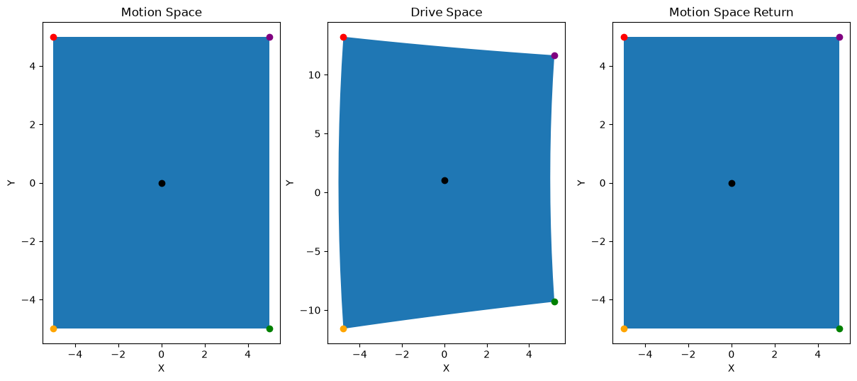
Are the returned motion space points “identical” to the starting points?

np.allclose(points, mpoints)

True

np.max(np.abs(points - mpoints))

np.float64(3.9968739429241396e-10)

The Algorithms

To start we will use \((e_0, e_1)\) to represent the drive space coordinates and \((x, y)\) to represent the motion space coordinates.

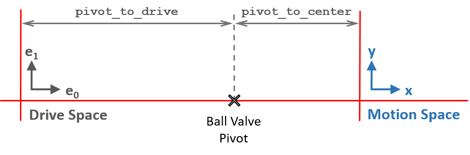
Top-Level Cartoon of the Drive and Motion Space Relationship

Note: The motion space x-axis points towards the the LaPD -X when the probe drive is deployed on the East side of the machine. This is why the East side operation requires mspace_polarity = [-1, 1], and the West side requires mspace_polarity = [1, 1].

Algorithm: Drive to Motion Space

The key parameter we need to determine to convert the drive space coordinates to the motion space coordinates is the angle \(\theta\), which is the angle the probe shaft makes with the horizontal. Let’s consider the following diagram…

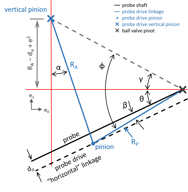
Drive Space Overview

Here…

• \(d_o\) = probe_axis_offset which is the perpendicular distance from the probe axis to the pinion location on the horizontal arm of the 6K probe drive.

• \(R_A\) = six_k_arm_length which is the length of the vertical hanging arm of the 6K probe drive.

• \(\beta\) is the angular drop of the pinion location from the probe drive shaft with respect to the ball valve

  \[tan\,\beta = \frac{d_o}{\texttt{pivot}\_\texttt{to}\_\texttt{drive}}=\frac{\texttt{probe}\_\texttt{axis}\_\texttt{offset}}{\texttt{pivot}\_\texttt{to}\_\texttt{drive}}\]

• \(R_P\) = pivot_to_drive_pinion the radial distance of the probe drive pinion from the ball valve pivot

  \[R_P^2 = d_o^2 + \texttt{pivot}\_\texttt{to}\_\texttt{drive}^2\]

• The vertical pinoin location above the horizontal is given by \(R_A - d_o + e_1\), assuming \(e_1=0\) when the probe shaft is horizontal.

• \(\gamma\) is the angle the vertical pinion makes with respect to the ball valve pivot and the horizontal

  \[\tan\,\gamma = \frac{R_A - d_o + e_1}{\texttt{pivot}\_\texttt{to}\_\texttt{drive}}\]

Now adopt a reference frame where the line intersecting the ball valve pivot and probe drive vertical (grey dashed above) is rotated to the horizontal and the ball valve is the origin. In this reference frame will use a coordinate system \((s_0, s_1)\). In this system the pinion point is located at the intersection of two circles:

1. The circle about the ball valve pivot of radius \(R_P\).

   \[R_P^2 = s_0^2 + s_1^2\]

2. The circle about the vertical pinion of radius \(R_A\).

   \[\begin{split}R_A^2 = (s_0 + L)^2 + s_1^2\\ \text{where}\; L^2 = (R_A - d_o + e_1)^2 + \texttt{pivot}\_\texttt{to}\_\texttt{drive}^2\end{split}\]

Solving this system of equations we can calculate the location of the pinion and, thus, the angle \(\phi\) depicted in the Drive Space Overview figure.

\[\tan^2 \phi = \left(\frac{2\,L\,R_P}{R_A^2-R_P^2-L^2}\right)^2 - 1\]

Knowing \(\phi\), the signed angle \(\theta\) can be expressed as

\[\theta = \gamma +|\beta|-|\phi|\]

Taking \(\theta\) and the radial projection of the probe into the motion space as \(r=D_C + e_0\), where \(D_C\) is the distans from the ball valve pivot to the motion space origin pivot_to_center, then the motion space coordinates can be expressed as

\[\begin{split}x = (\cos\theta) \, e_0 + D_C \,(\cos\theta-1)\\ y = (-\sin\theta)\, e_0 - D_C \,\sin\theta\end{split}\]

and expressed as the _matrix_to_motion_space

\[\begin{split}\begin{bmatrix} x \\ y \\ 1 \end{bmatrix} = \begin{bmatrix} \cos\theta & 0 & D_C \, (\cos\theta - 1)\\ -\sin\theta & 0 & -D_C \, \sin\theta\\ 0 & 0 & 1\\ \end{bmatrix} \begin{bmatrix} e_0 \\ e_1 \\ 1 \end{bmatrix}\end{split}\]

Obviously this not a perfectly clean expression since \(\theta\) depends on \(e_1\). However, this is the expression that must be used to work with the archatecture designed int BaseTransform.

Algorithm: Motion to Drive Space

In order to convert from the motion space to the drive space the key parameter to determine is the location of the probe drive pinion. Again this boils down to determining the angle \(\theta\), since the pinion is always a distance \(R_P\) from the ball valve pivot and at an angle of \(\theta - |\beta|\).

Knowing the motion space coordinates \((x, y)\) the angle \(\theta\) can be written as..

\[\tan\theta = -\frac{y}{D_C + x}\]

Then the probe drive pinion is located at the following position with the ball valve coordinate system \((s_0, s_1)\)

\[\begin{split}s_0 = -R_P \cos(\theta - |\beta|)\\ s_1 = R_P \sin(\theta - |\beta|)\end{split}\]

Now we can determine the angle \(\alpha\) in which the probe drive arm leans forward.

\[\sin\alpha = \frac{\texttt{pivot}\_\texttt{to}\_\texttt{drive} + s_0}{R_A} = \frac{\texttt{pivot}\_\texttt{to}\_\texttt{drive} - R_P \cos(\theta - |\beta|)}{R_A}\]

\[\cos\alpha = \frac{R_A - d_o + e_1 - s_1}{R_A} = \frac{R_A - d_o + e_1 - R_P \sin(\theta - |\beta|)}{R_A}\]

Now we can cast the drive space coordinates as

\[\begin{split}e_0 = \frac{1}{\cos\theta}x + D_C\left(\frac{1}{\cos\theta}-1\right)\\ e_1 = R_A (\cos\alpha - 1) + d_o + R_P \sin(\theta - |\beta|)\end{split}\]

where

\[\begin{split}\sin\alpha = \frac{\texttt{pivot}\_\texttt{to}\_\texttt{drive} - R_P \cos(\theta - |\beta|)}{R_A}\\ \tan\theta = -\frac{y}{D_C + x}\end{split}\]

The does yield a rather ugly, but functional, transformation matrix of

\[\begin{split}\begin{bmatrix} e_0 \\ e_1 \\ 1 \end{bmatrix} = \begin{bmatrix} \frac{1}{\cos\theta} & 0 & D_C \, \left(\frac{1}{\cos\theta} - 1\right)\\ 0 & 0 & R_A (\cos\alpha - 1) + d_o + R_P \sin(\theta - |\beta|)\\ 0 & 0 & 1\\ \end{bmatrix} \begin{bmatrix} x \\ y \\ 1 \end{bmatrix}\end{split}\]